Marching Squares in Python
Marching Squares is an algorithm that extracts edges as line segments from a 2D grid of values. The values could come from anywhere – a volumetric function or discrete data, for example. This algorithm is useful whenever edge or boundary data is needed (such as toolpaths or G-Code for a 3D printer).
Marching Squares is a 2D version of Marching Cubes, which is a very common algorithm for extracting surfaces as triangle meshes from implicit functions or discrete 3D data like MRI and CT scans.
A repository with some demo code can be found here.
Motivation
Let’s look at an example to make the need for this a bit clearer:
I have an image of a circle. We clearly see that it’s a circle, but it’s really just a grid of values from 0 to 255 (x3 for red, green, and blue). What if we want a smooth path or series of line segments to trace out the shape of the circle?
Okay, the equation of a circle is easy, so it still doesn’t seem too hard. What about more complex, arbitrary shapes for which we don’t have a direct equation?
Even if we have an equation, that doesn’t necessarily mean it’s easy to convert into a toolpath. SDFs (signed distance functions) are a good example. The SDF of a circle is: sqrt(x2 + y2) - r = 0. This is great when we need information about the inside and outside of the circle but not so great if we just want to trace the perimeter.
Basic Steps
For each square in a uniform 2D grid:
- Sample a function (or data) at each corner point
- Create four binary values using these four values and a threshold (typically zero). These values represent a state (a lookup ID). Since the number of binary combinations of the four corners is finite (2^4=16), a lookup table can be used to construct these edges very quickly.
- Use this ID to look up the connections between edge midpoints to make based on the edge table.
- Insert the edges from the table into a list and move to the next square
For those who aren’t very familiar with binary (like I wasn’t), it’s pretty simple. From right to left, each 0 or 1 represents an increasing power of two: …23222120. The integer value is the sum of the powers multiplied their corresponding binary value. This means any number, even or odd, can be represented this way. There are conventions for handling negative numbers and decimal places but those don’t affect this use case.
0010: (8*0)+(4*0)+(2*1)+(1*0) = 20111: (8*0)+(4*1)+(2*1)+(1*1) = 7
Below is the lookup table in a Python dictionary:
1
2
3
4
5
6
7
8
9
10
11
12
13
14
15
16
17
18
STATES = {
    0 : [],
    1 : [[2,3]],
    2 : [[1,2]],
    3 : [[1,3]],
    4 : [[0,1]],
    5 : [[0,3], [1, 2]],
    6 : [[0,2]],
    7 : [[0,3]],
    8 : [[0,3]],
    9 : [[0,2]],
    10 : [[0,1], [2, 3]],
    11 : [[0,1]],
    12 : [[1,3]],
    13 : [[1,2]],
    14 : [[2,3]],
    15 : []
}
Example
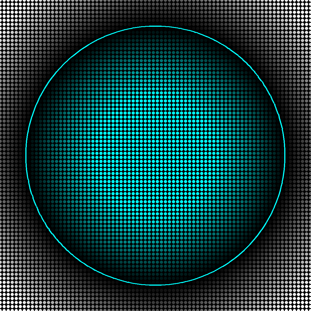
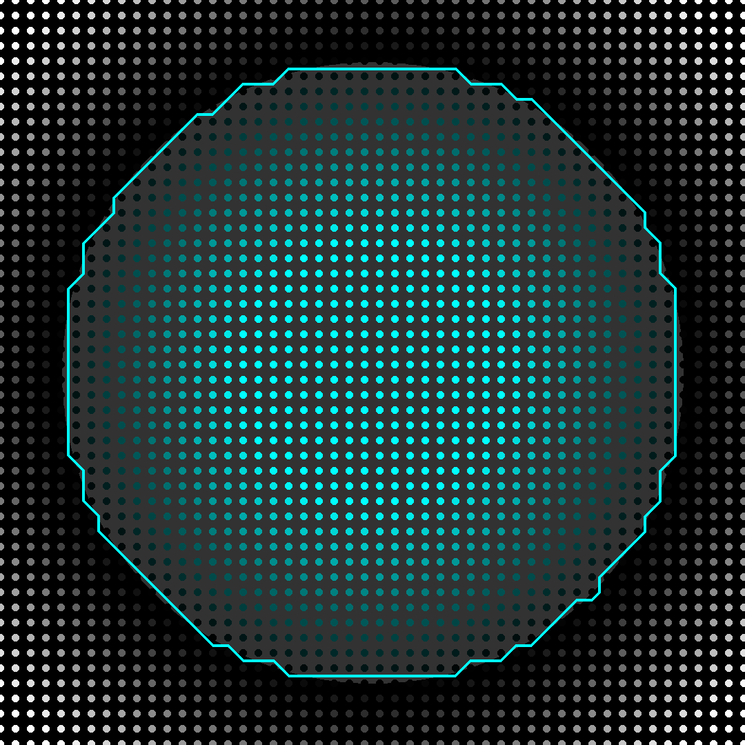
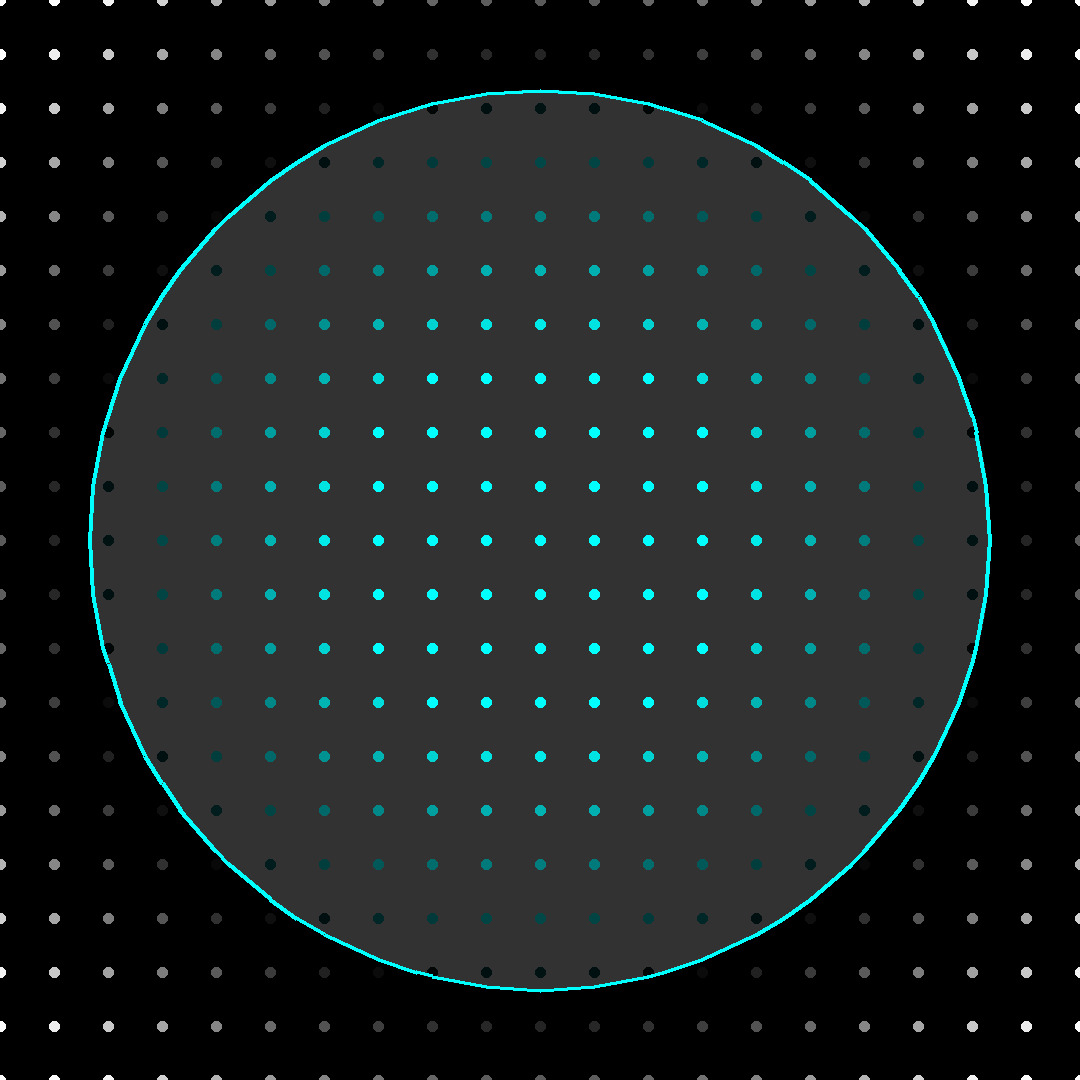
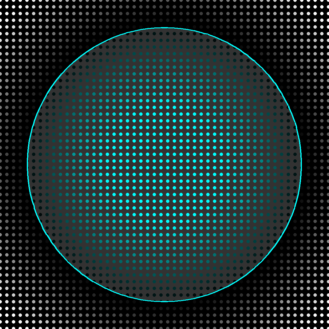
Extracting the edges of an implicit circle defined by a signed distance function. The circle’s boundary is where the function is equal to zero. The dot colors represent the distance values at each sampling location and the cyan lines are the extracted boundary.
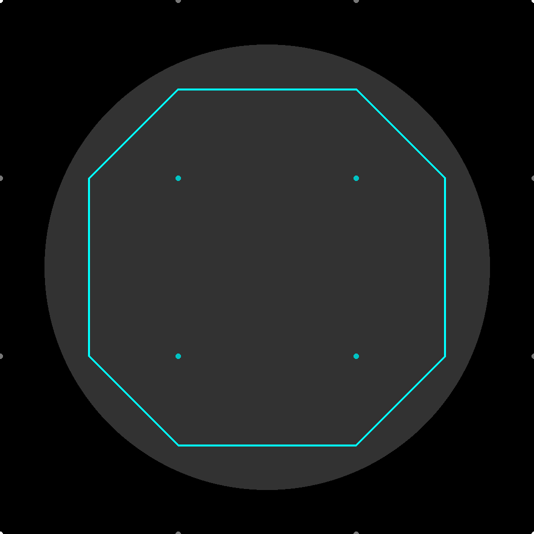
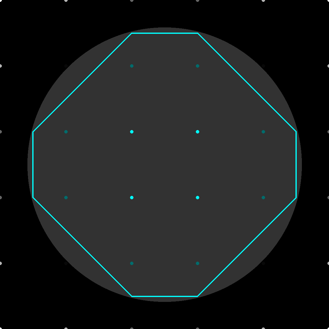
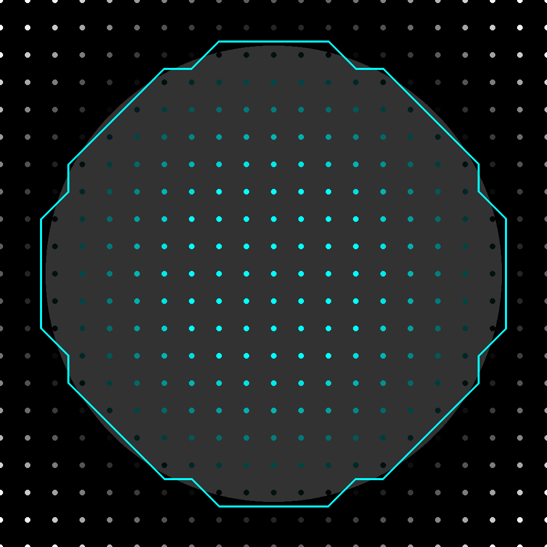
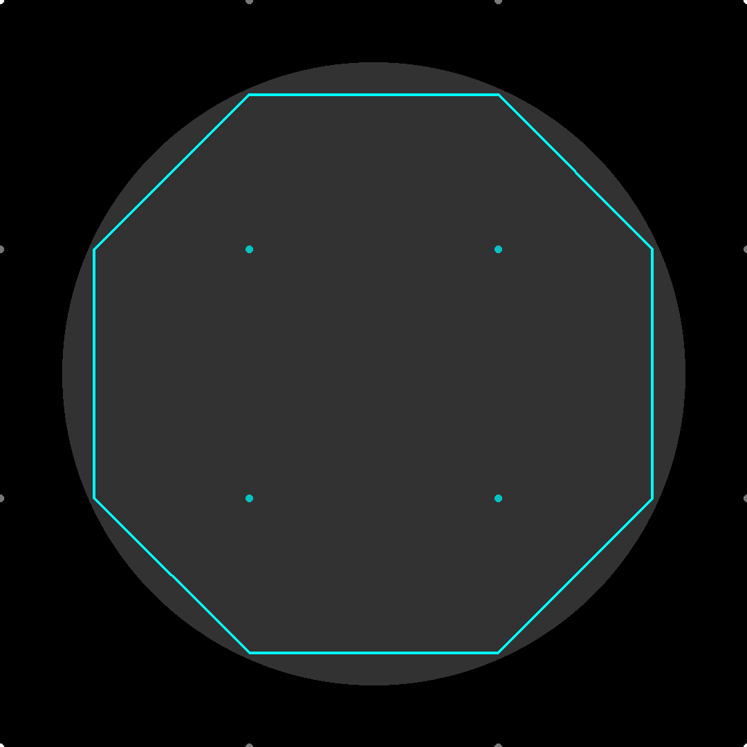
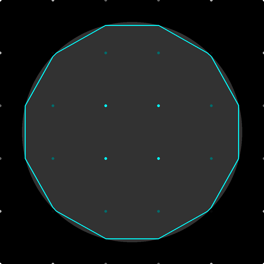
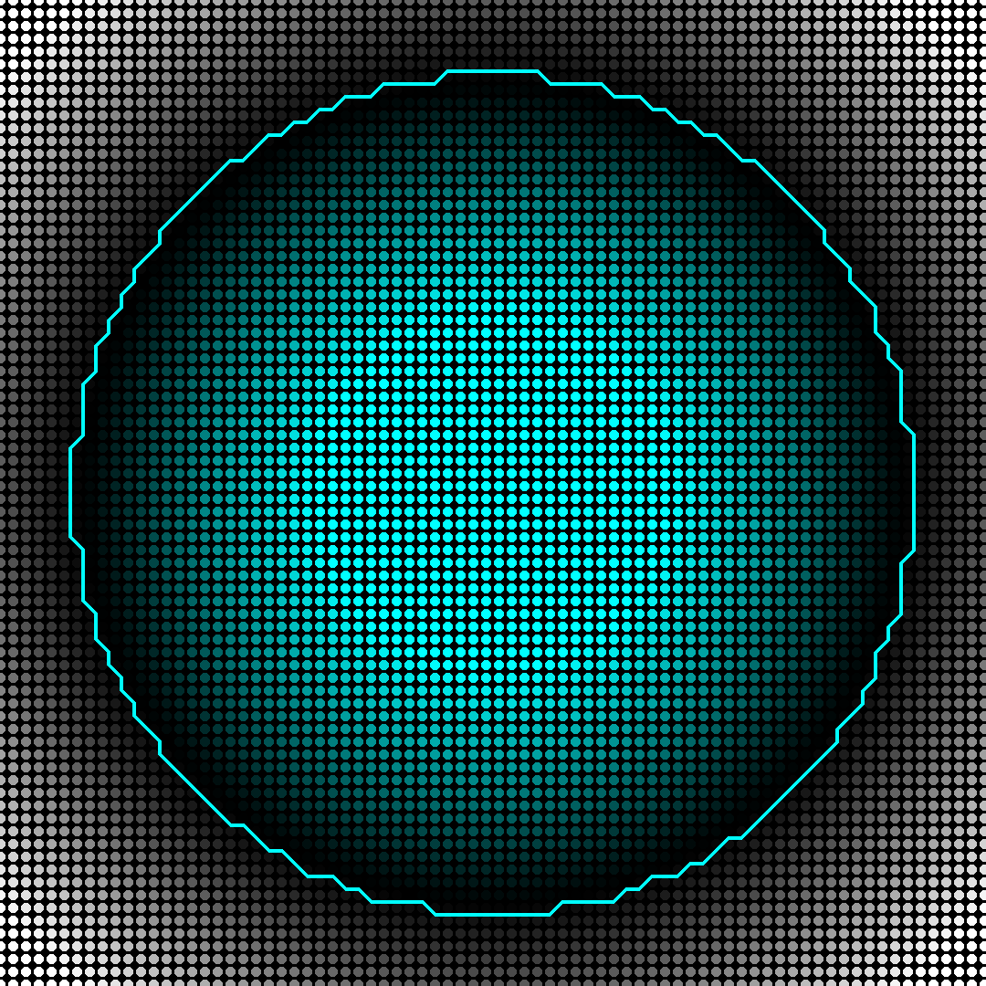
The size of the sampling grid determines the “resolution” and thus the maximum deviation from the “actual” boundary the resulting edges will have. The maximum possible deviation from the base surface is sqrt(2) * grid size. Here is a comparison of different sample grid resolutions:
*Note: The only output of Marching Squares is the cyan line segments. The rest of what’s shown in the images is for visualization only. The cyan-black-white gradient represents the negative-zero-positive distance field.
Interpolation
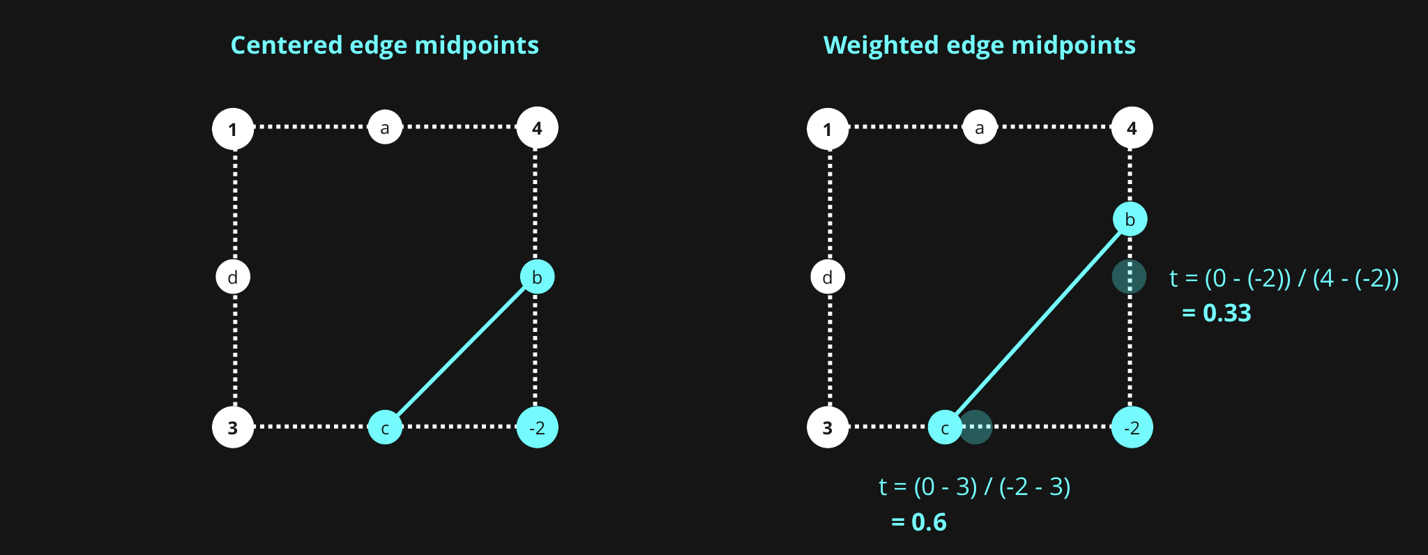
Linear interpolation with weighted sample points is used to shift the vertices of the new edges to more closely follow the actual shape. If only midpoints on each square edge are used then the resulting line segments are horizontal, vertical, or angled at 45 degrees.
This can improve the results fairly dramatically:
In my example, I find the interpolation factor with this bit of code:
1
2
3
def find_lerp_factor(v0, v1, iso_val):
    t = (iso_val - v0) / (v1 - v0)
    return max(min(1, t), 0)
Discrete Data
Discrete input data, such as with an image, can be used as described in the intro. The drawback is, if the data is discontinuous, linear interpolation won’t work directly to achieve a smooth boundary. A quick and dirty way of getting around this is applying a box or gaussian blur. This can come at the cost of some accuracy, which may or may not be okay depending on the application. Note that the black band at the bottom of the balloon is enclosed in the right image; this is because of a combination of the box blur and sample resolution.
Let’s use marching squares to extract the regions of this image with a lot of red:
References:
